Dating a Super Tree using the FBD model
Thanks to David Černý for his help developing this code.
In paleobiology there are often situations where we want to date a supertree, or any tree for which we do not have any character data associated with taxa at the tips. This is commonly carried out in MrBayes, though it is also possible to do in RevBayes.The following tutorial provides sample code for dating a super tree of Theropod dinosaurs in Revbayes using the Fossilized Birth death model. The data is from Tasimov et al. (in prep) and is of 66 taxa with ages ranging from Middle Jurassic to Late Cretaceous.
Note: This tutorial uses both R and RevBayes for steps of the inference. RevBayes is under active development and will eventually provide a approach to carry out the full analysis. Coming soon-ish……
Organise you code
As with any analysis it is important to set up you directories correctly. You should have a scripts and a data folder. The trees and fossils ages can be downloaded here
1. Time-scaling the tree in R
For this inference Revbayes requires a time-scaled tree as the input.
We can carry out this time-scaling in R studios. The exact method of
time scaling used here should not have an impact on the over
all inference results. We can use the R package paleotree
to do this. Additionally, if your tree has polytomies we need to provide
RevBayes with a fully resolved tree as the initial tree and the original
tree is then supplied as the so called backbone tree. In this way the
polytomies can be resolved by leveraging the temporal information during
the FBD analysis.
Load relevant r packages
library(paleotree)
library(phytools)
library(phangorn)
library(ape)
We first need to read in our age data and create a matrix of ages required for the time scaling method
taxa_ages <- read.table("data/ages.csv", header = T)
rownames(utaxa_ages) <- taxa_ages[,1]
dinoRanges <- taxa_ages[,2:3]
We can read in our tree
phy <- ape::read.tree("data/dino.tree")We then borrow a function from Liam Revell’s website for randomly resolving polytomies
resolveRandom<-function(tree){
  while(!is.binary(tree)){
    nodes<-1:tree$Nnode+Ntip(tree)
    Nchildren<-function(node,tree) length(Children(tree,node))
    nchilds<-sapply(nodes,Nchildren,tree=tree)
    node<-nodes[which(nchilds>2)[1]]
    tree<-sample(resolveNode(tree,node),1)[[1]]
  }
  tree
}


Binary_tree <- resolveRandom(phy)
Using the function timePaleoPhy in the PaleoTree package
we can estimate branch length with units of time for our trees (the
original tree and the fully resolved, or binary, tree). The
type variable here refers to the time scaling appraoch
used. We are using “mbl” which ensures that there are no zero branch
lengths, which is a common result when using the “basic” method.
tt_polytomy <- paleotree::timePaleoPhy(tree = phy, timeData = dinoRanges, type = "mbl", randres = FALSE,
                                       ntrees = 1, plot= T, vartime = 2)


tt_binary <-  paleotree::timePaleoPhy(tree = Binary_tree, timeData = dinoRanges, type = "mbl", randres = FALSE,
                                      ntrees = 1, plot = T, vartime = 2)
Now we can write the trees to file to use them for our FBD inference
write.tree(tt_polytomy,"data/dated_backbone.tre")
write.tree(tt_binary,"data/dated_initial.tre")
2. FBD inference in RevBayes
Below I will provide the code for estimating divergence times of a super tree using the FBD model. It is important to note that this code works by fixing the fossil ages. This has been shown to be problematic, see Barido-Sottani et al 2020, however is currently the only practical implementation. The new release of RevBayes will allow you to estimate these ages, so keep an eye out for that!
As with any analysis it is helpful to give it a name
analysis_name = "Palss_2024"We can then read in our age information
### read in the age infromation
taxa <- readTaxonData("data/ages.csv")
Read in our backbone tree (i.e., our original tree with polytomies)
## read in the backbone tree - the one with ploytomies
bb <- readTrees("data/dated_backbone.tre")[1]
As there is no explicit information in our newick string about the age of the tree we need to offet it by the age of the youngest fossil
## offset the ages by the age of the youngest tip
bb.offset(98)
We can do the exact same for the starting tree
init <- readTrees("data/dated_initial.tre")[1]
init.offset(98)
We initialize vectors for our moves and monitors
moves = VectorMoves()
monitors = VectorMonitors()
We can then set the priors on our FBD paramters: speciation, extinction, and sampling
speciation_rate ~ dnExponential(10)
extinction_rate ~ dnExponential(10)

moves.append( mvScale(speciation_rate, lambda=0.01, weight=1) )
moves.append( mvScale(speciation_rate, lambda=0.1,  weight=1) )
moves.append( mvScale(speciation_rate, lambda=1.0,  weight=1) )

moves.append( mvScale(extinction_rate, lambda=0.01, weight=1) )
moves.append( mvScale(extinction_rate, lambda=0.1,  weight=1) )
moves.append( mvScale(extinction_rate, lambda=1,    weight=1) )


psi ~ dnExponential(10)
moves.append( mvScale(psi, lambda=0.01, weight=1) )
moves.append( mvScale(psi, lambda=0.1,  weight=1) )
moves.append( mvScale(psi, lambda=1,    weight=1) )
We can keep track of parameters of interest during the analysis
diversification := speciation_rate - extinction_rate
turnover := extinction_rate/speciation_rate
As our tree is fully extinct we can set rho, the probability of extant species sampling, to zero
rho <- 0The origin age is set using a uniform prior on the start of the Triassic and the oldest fossil
origin_age ~ dnUniform(170.9, 251)
moves.append( mvSlide(origin_age, delta=0.1, weight=5) )
Having defined all our parameters we can create our FBD object
fbd_dist = dnFBDP(originAge=origin_age, lambda=speciation_rate, mu=extinction_rate, psi=psi, rho=rho,taxa=taxa)The FBD tree is constrained using both of the time trees
fbd_tree ~ dnConstrainedTopology(fbd_dist, backbone=bb, initialTree=init)

moves.append( mvFNPR(fbd_tree, weight=15.0) )
moves.append( mvCollapseExpandFossilBranch(fbd_tree, origin_age, weight=6.0) )
moves.append( mvNodeTimeSlideUniform(fbd_tree, weight=40.0) )
Record the number of sampled ancestors
num_samp_anc := fbd_tree.numSampledAncestors()Define our model
mymodel = model(fbd_tree)Define some monitors
# 1. for the full model #
monitors.append( mnModel(filename="output/" + analysis_name + "_dino.log", printgen=10, exclude = ["F"]) )

# 2. the tree #
monitors.append( mnFile(filename="output/" + analysis_name + "_dino.trees", printgen=10, fbd_tree) )

# 3. and a few select parameters to be printed to the screen #
monitors.append( mnScreen(printgen=1000, origin_age) )
Finally, initialise and run our inference
# Initialize the MCMC object #
mymcmc = mcmc(mymodel, monitors, moves, nruns=2, combine="mixed")


mymcmc = mcmc(mymodel, monitors, moves)
mymcmc.run(generations=10000)
Create a summary tree
trace = readTreeTrace("output/" + analysis_name + "_dino.trees")
mccTree(trace,"output/" + analysis_name + "_dino_mcc.tre", positiveBranchLengths = TRUE)
Note: this will not converge! The chain needs to be run for a lot longer, but that is ok for the purposes of this tutorial.
3. Tree visualization in R
We can plot our time tree in R using the R package
RevGadgets. This R package provides lots of cool ways for
processing the output of a phylogentic inference in RevBayes, for more
information see
library(RevGadgets)
file <- "output/Palss_2024_dino_mcc.tre"
FBD_tree <- RevGadgets::readTrees(paths = file)
As before we need to include our offset, so we add 98 to the posterior of tree
FBD_tree[[1]][[1]]@data[["age_0.95_HPD"]]<-
  lapply(FBD_tree[[1]][[1]]@data[["age_0.95_HPD"]], function(x) x + 98)
Create our plot
p <- plotFBDTree(tree = FBD_tree,
            timeline = T,
            geo_units = "epochs",
            tip_labels_italics = T,
            tip_labels_remove_underscore = T,
            tip_labels_size = 1,
            tip_age_bars = T,
            node_age_bars = T,
            age_bars_color = "blue",
            label_sampled_ancs = TRUE,
            line_width = 0.5,
            age_bars_width = 0.5)
Add our offset to the tree object and plot
p$data$x <- p$data$x - 98
p
You should end up with a tree like this:
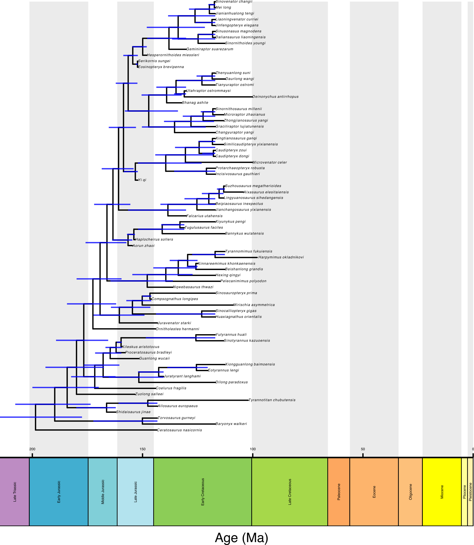
You can play with the plotting function to make this tree look nicer! Download the complete scripts for this tutorial here
4. Skyline FBD
We can relax the assumption of constant speciation, extinction, and fossil sampling in an FBD analysis by using a skyline model. This model allows rates to vary in a piece-wise manner across different geological intervals. Essentially, creating time-bins as in common with many paleontological methods. To do this you need to define your timeline and create a vector of your rates for each bin.
We can edit the existing FBD.rev file as as follows (copy the FBD.rev file and rename it).
Update the name of the analysis.
analysis_name = "Palss_2024_skyline"Define the time line specifying the intervals. We will set four time bins here, representing the middle Jurassic, Late Jurassic, Early Cretaceous, and Late Cretaceous.
timeline <- v(100.5, 145, 163.5)You can remove how we defined speciation, extinction and fossil sampling from this new skyline analysis. We can then loop through the different time bins to estimate rates for each of them.
alpha <- 10

for(i in 1:(timeline.size()+1))
{
    extinction_rate[i] ~ dnExp(alpha)
    speciation_rate[i] ~ dnExp(alpha)
    psi[i] ~ dnExp(alpha)

    diversification[i] := speciation_rate[i] -  extinction_rate[i]
    turnover[i] :=  extinction_rate[i]/speciation_rate[i]

    moves.append( mvScale(extinction_rate[i], lambda = 0.01) )
    moves.append( mvScale(extinction_rate[i], lambda = 0.1) )
    moves.append( mvScale(extinction_rate[i], lambda = 1) )

    moves.append( mvScale(speciation_rate[i], lambda = 0.01) )
    moves.append( mvScale(speciation_rate[i], lambda = 0.1) )
    moves.append( mvScale(speciation_rate[i], lambda = 1) )

    moves.append( mvScale(psi[i], lambda = 0.01) )
    moves.append( mvScale(psi[i], lambda = 0.1) )
    moves.append( mvScale(psi[i], lambda = 1) )
}
Our FBD model then uses a vector of values for these rates
fbd_dist = dnFBDP(originAge=origin_age, lambda=speciation_rate, mu=extinction_rate, psi=psi, rho=rho, taxa=taxa, timeline=timeline)Nothing else in the script needs to be changed for this analysis. Here we have all three parameters varying, however, we could choose to fix one, for example fossil sampling, and then just allows speciation and extinction to vary though time.